Hold'em or Fold'em?: Simulating Poker Deals

Introduction

If you are like me, you know enough about playing Hold'em to have a good time with friends, but not enough to win consistently or to bet competently.  Looking at strategies and tips for betting left me a little confused, so I turned to what I know to help me: simulation.

Through the use of simulated poker deals, I figured I could derive some principles for how to understand the strength of my hand in any given deal.  And whether or not I should hold'em or fold'em.

Obviously, the following has nothing to say about bluffing, or when or what to bet.  I merely offer some observations about which hands are likely to win based on the probabilities of hand distributions.  You can use these observations to develop your own strategies for how to win.

Hand Distributions

The following is a table of the distribution of hands over 100,000 simulated deals for a single player.  That is, it contains the likelihood that you will get a particular kind of hand on any given deal with your two dealt cards in combination with the five community cards.

Player1	Count	Percentage
9. One Pair	44239	44.24
8. Two Pair	23279	23.28
10. High Card	17791	17.79
7. Three of a Kind	4918	4.92
6. Straight	3968	3.97
5. Flush	2821	2.82
4. Full House	2642	2.64
3. Four of a Kind	174	0.17
2. Straight Flush	145	0.15
1.Royal Flush	23	0.02

I ran this simulation several times and the results were similar each time.  What I found most interesting is that it is less likely to only have a high card hand than it is to have a one pair or a two pair hand.  This is surprising because a high card is ranked lower than a one pair or a two pair hand.  One would expect that the ranking of hands would follow their likelihood of occurring.  This is the case for all hands, except for the single high card hand.

What does this mean practically? Well, one has 68% chance of getting a one pair or two pair.  Each individually is more likely than a single high card hand.  Overall, one has an 82% chance of not having a single high card hand.  So it is unlikely that one will only have a high card hand after all of the cards are dealt.

Chances Against One Other Player

Below is a table of how often Player1 won, tied, or lost whenever Player1 had the specified hand dealt.  This is over 100,000 simulations.  Note that I do not use tie-breaking rules to determine a final winner.  Instead, a tie designates that Player1 and Player2 had the same kind of hand (although one or the other may actually have won given the tie breaking rules).  I do this to simplify this initial round of analysis.  Also note that when I use the word "win", I am excluding ties in the calculation (see below), as I am concerned with wins versus losses.

Player1	Lose	Tie	Win	Win/(Win+Loss)	Tie/All
1.Royal Flush	0	0	23	1.00	0.00
2. Straight Flush	0	5	140	1.00	0.03
3. Four of a Kind	0	24	150	1.00	0.14
4. Full House	40	409	2193	0.98	0.15
5. Flush	80	620	2121	0.96	0.22
6. Straight	150	768	3050	0.95	0.19
7. Three of a Kind	733	1001	3184	0.81	0.20
8. Two Pair	3274	8857	11148	0.77	0.38
9. One Pair	14830	20968	8441	0.36	0.47
10. High Card	11655	6136	0	0.00	0.34

Some observations:

• A Royal flush, straight flush, and four of a kind always won or tied.  There is practically 0% chance of losing.
• When calculating win/(win+loss), a full house, flush, and straight won 98%, 96%, and 95% of the time, respectively.  In other words, there is a very small chance of losing.  One is more likely to tie than to lose (15%, 22%, and 19% chance of tying, respectively).
• When calculating win/(win+loss), three of a kind and two pair won 81% and 77% of the time, respectively.  Chances of tying are 20% and 38%, respectively.  One has a small chance of losing.  One is more likely to win or tie.
• When calculating win/(win+loss), one pair won only 36% of the time.  One pair tied 47% of the time.
• A high card always loses or ties.  Chances are 34% for a tie.

Given the foregoing, it is reasonable to suggest that if one has a two pair or more, one should stay in play.  Why?  Because chances are that one has the best hand.  Of course, you probably want to have a high two pair (AA or KK) and don't want that high pair in the community cards.  But overall, if you have a two pair or better, you should stay in. 

On the other hand, if you have a one pair or high card only, you should fold (or be really good at bluffing).  You are more likely to lose (or tie) than win.

Chances Against Two Other Players

Things change a little with two other players.  Here is the table of how often Player1 won, tied, or lost when two other players were in the game:

Player1	Lose	Tie	Win	Win/(Win+Loss)	Tie/All
1.Royal Flush	0	0	33	1.00	0.00
2. Straight Flush	0	5	150	1.00	0.03
3. Four of a Kind	0	25	156	1.00	0.14
4. Full House	31	765	1684	0.98	0.31
5. Flush	88	647	2220	0.96	0.22
6. Straight	170	777	3123	0.95	0.19
7. Three of a Kind	1538	107	3238	0.68	0.02
8. Two Pair	3338	16649	3439	0.51	0.71
9. One Pair	24953	19101	0	0.00	0.43
10. High Card	17763	0	0	0.00	0.00

Some observations:

• A Royal flush, straight flush, and four of a kind always won or tied.  There is practically 0% chance of losing.
• A full house, flush, and straight won 98%, 96%, and 95% of the time, respectively.  So very little has changed in that regard.  However, one is much more likely to tie now in a full house (31%).
• Three of a kind and two pair won only 68% and 51% of the time, respectively.  Chances of tying go down to 2% and up to 71%, respectively.  These hands are much less likely to win now.
• One pair won 0% of the time and tied 43% of the time.
• A high card always loses and never ties.

With the addition of one more player, the higher ranking hands (1-6) change very little.  However, three of a kind and two pair are no longer largely dependable for a win.  And a one pair or high card are guaranteed losses.  Given this, you need a straight or better for a relatively sure thing.  Be prepared for bluffing and a uneasy fight if you only have two pair or a three of a kind.

Chances Against Five Other Players

Finally, consider a game starting with 6 players total.  What does Player1 need now to have the best hand among the group?  Here is the table of how often Player1 won, tied, or lost when five other players were in the game:

Player1	Lose	Tie	Win	Win/(Win+Loss)	Tie/All
1.Royal Flush	0	1	21	1.00	0.05
2. Straight Flush	0	6	153	1.00	0.04
3. Four of a Kind	0	24	157	1.00	0.13
4. Full House	43	848	1723	0.98	0.32
5. Flush	105	643	2088	0.95	0.23
6. Straight	166	771	3040	0.95	0.19
7. Three of a Kind	1676	99	3054	0.65	0.02
8. Two Pair	3289	16993	3442	0.51	0.72
9. One Pair	25147	19029	0	0.00	0.43
10. High Card	17482	0	0	0.00	0.00

Some observations:

• A Royal flush, straight flush, and four of a kind always won or tied.  There is practically 0% chance of losing.  This is largely the same.
• A full house, flush, and straight won 98%, 95%, and 95% of the time, respectively.  So this is practically the same. One's chances of tying with a full house are about the same too (32%).
• Three of a kind and two pair remain practically the same, 65% and 51%, respectively.  Chances of tying are also the same.
• One pair stays the same.
• A high card stays the same.

This is a very interesting result.  I would have thought that as the number of players increases, one's chances of losing increase, and hence, the need for an even better hand to win.  But the probabilities are practically the same against two players as against five players.  The advice stays the same.

 

Conclusion

In summary, here are some general takeaways:

• Expect at least a pair to have been dealt to you after all community cards have been dealt.
• Against one other player, (ignoring ties) two pair is generally good enough to win (79%).  Anything above and including a straight is practically guaranteed to win.
• Against two to five other players, (ignoring ties) expect to win half the time with two pair, two-thirds of the time with three of a kind, and almost all the time with a straight and above.

Good luck!

Visualizing Data Science

Linked is a presentation I put together for TDWI Boston for the "Advanced Topics in Data Visualization" session.  Enjoy!

https://www.slideshare.net/fullscreen/51147149/1

POS News Update: Automatically Tweeting Using R

Introduction

I am fond of automation.  Why?  Because if I can automate something, then I don't have to do it manually, and that saves me time.  It also saves me emotional energy if it does a task that I really don't want to do. So automation can save me time and energy, particularly for unpleasant tasks.

One unpleasant task (at least for me) is that of self-promotion.  Nowadays it is a wise career move to continually post links and comment through Twitter, LinkedIn, Yammer, and various other job-related social media.  It is to one's advantage to remain engaged in hot topics in one's field and to demonstrate knowledge by posting insightful comments.  By doing so, one demonstrates that one is a leader in the field (and worthy of pursuit in hiring and career advancement).

But we know that such self-promotion can be very time consuming, and perhaps unpleasant for us, even though it is beneficial for our careers.  How can we have our cake and eat it too?  Enter in automation. I thought, if I could automate some of this "self-promotion", I could be more actively engaged in the community AND also free up some time for myself.  Plus, it would be a fun avenue of personal research for advancing my skills.

Automating Twitter "News" Updates

I am not very active in Twitter (at all), so I thought this would be a good place to start with an automation experiment.  What would I Tweet?  I wanted to explore Natural Language Processing a bit, so I eventually settled on doing the following:

1. Gather the latest Google News headlines.
2. Use Parts of Speech tagging to break down each headline into parts of speech.
3.  Swap out words in each headline for another word with the same parts of speech tag (e.g, swap a noun for a different noun).
4. Pick a headline that reads the most like a sentence
5. Post the headline to Twitter automatically on a regular schedule

R packages Used

For those that are interested, I used the following packages:

• httr - used to authenticate the twitter api and create my twitter token.  Follow the code here to replicate.  Used the POST() function to send my update to Twitter.  See here for code.
• rvest - used to get the Google News headlines.
• openNLP - used to do the POS tagging for the headlines and sentence evaluation.

I used Task Scheduler to run a batch file that ran the R file I created.  See here for the process to automate this.

Results

The results are mixed.  Sometimes the headlines make sense and sometimes they don't.  I suppose this isn't very surprising.  Headlines are difficult to analyze because they are not complete sentences.  As such, the POS tags are often wrong.  Additional work is needed to have better swaps, and consequently, more readable headlines.  However, my larger goal of being able to automatically post Tweets was successful, and may prove useful in the future for other projects of mine.

Here is my favorite post so far:

POS News Update: 'HUCKABEE MUSK, STEPHEN HAWKING WANT TO SAVE THE WEBSITE FROM LETTUCE CONCERNS'

You can see these for yourself by following me on Twitter at @philanalytics

From Trolley Problems to Transactional Databases: My Move from Academia to Business

This post was originally written for use at VersatilePhdD.com with help from the founder of Versatile PhD, Paula Chambers.  Versatile PhD is a site devoted to helping graduate students and PhDs transition to non-academic careers and to be successful in them.  The site provides a community of support, job postings, and transition success stories, among other resources for those thinking about such a transition.

Below is an edited version of my own success story.  Enjoy!

-------------------------------------------------------------------------------------------------------------------------

            Early in the spring of 2011, my first year of a two year MA program, I began to have serious doubts about entering into a teaching career and continuing on into a PhD program in Philosophy.  I became more aware of the job market and what lay ahead of me if I wished to continue studying philosophy at the professional level.  Faced with the prospect of many years of graduate study, followed by a long struggle to find a tenure-track position with little financial incentive, even at the peak of my career, I began to doubt whether this was the right path for my career to take.

I started to discuss my situation with professors and classmates.  Fortunately, the professors I talked with were understanding and sympathetic.  They affirmed that my concerns were legitimate and discussed their own experiences of struggle in obtaining secure teaching positions, the pressure to publish, the challenge of teaching unmotivated students, leftover debt, and the lack of choice of where to live.  Why then did they continue to teach?  Simply put, my professors were so passionate about philosophy that they could not imagine doing anything else.  They would sacrifice money, drive long distances to teach, and move away from friends and family, all so that they could continue to study and teach philosophy for a living.  In other words, doing philosophy was their highest priority.  Like my professors, many of my classmates felt the same way.  I recall that one of my classmate’s idea of taking a break from writing a metaphysics paper was to read an epistemology book.  He, like many others, could not get enough philosophy and didn’t want to do anything else.

Given the sacrifices and choices I would have to make, I realized that, unless I was also passionate about and fully committed to studying and teaching philosophy, I should not do it professionally.  That is, unless I could not conceive of doing anything else as a career besides philosophy, I should choose to do something else.  If I could conceive of alternatives, it was probably better for me to pursue those.  Consequently, later that spring, I chose to stop looking into prospective PhD programs and began to look into alternative career paths. 

Generally, my professors and classmates were supportive of my decision to not apply for PhD programs and to pursue other options.  Some professors were a little disappointed as they recognized that I could have placed well and been successful.  And some classmates, when I voiced my reasons for not continuing on to the PhD level, pushed back and tried to persuade me to stick with philosophy.  Nevertheless, I mostly received support for my decision as the best decision for me.  My department head even told me that his view of success for graduating MA students was not that they would necessarily go into top ranked PhD programs and teach in philosophy.  Instead, it was that each student would graduate with valuable skills in writing, reasoning, and analysis that would make him or her successful in whatever career path the student chose. Thus, I largely had support to move forward in pursuing other options.

            Having come to peace with my decision to leave academia after completing my MA, I needed an alternative career path.  But what would I do now?  Discussing my situation with a close college friend, he suggested I intern with his dad’s database consulting company, over the summer.  As I began my internship, I discovered that many technical skills were simply applied philosophy skills I had already learned.  For example, object oriented programming was simply applied logic, and SQL querying was simply applied set theory.  I had a BA in Mathematics and a logic background from my philosophy training, so the transition to learning SQL and understanding database design and technology was relatively smooth.

The internship went well and I decided to continue on in that direction.  When I returned for my second year of graduate study in philosophy, I took introductory C++ programming, advanced computer programming, and continued to read about database design, programming, and SQL querying on my own.  As such, upon graduation with my MA in spring 2012, I was immediately marketable as an entry level database administrator.

            I continued on as an intern with my previous company that summer until I could be placed on a project.  I worked on internal projects, met with prospective clients, helped my coworkers, and continued to study and develop the skills I would need for this line of work.  Meanwhile, my boss continued to look for opportunities to place me on a project.  In July 2012, one of my friend’s network connections let him know of an available contract position on his team at Microsoft.  My friend then let me know about the position and suggested I consider it and meet with the client for an interview later that day, which I did.

The interview went very well.  The client knew of me from several of my friends and had no concern about my ability to do the work.  Our commonality in having an MA in philosophy probably cemented the deal as he knew I would be able to think intelligently and creatively in dealing with the day to day work requirements.  And, thanks to my internship, classes, and independent study, I had the technical expertise to actually do the work.  In any case, I was offered the job and I accepted.

While continuing to develop my skills on the job, I enrolled in a certificate program in Data Science through the University of Washington.  Through this program I learned more about database design and administration, Business Intelligence, data mining, and predictive analytics.  Now, having graduated from the program and through my experience on the job and continued learning off the job for over a three years, I have become marketable as a database administrator, business intelligence consultant, and data scientist.  Thankfully, and in great contrast to academic teaching at the college and university level, these positions are widely available and those that can fill them are greatly in demand.  As such, I continue to consult in the Seattle area as part of a consulting firm, working in these areas of data management and data analysis.

Some specific practical advice for getting a nonacademic job.  First, you need to prepare yourself technically.  My experience, and the experience of others I know, is that in the business and technology world you don’t need a degree in something to be hired to do it.  You just need to know how to do it.  So continue your education by reading books, taking continuing education courses, doing certificate programs, and taking classes outside your degree while still doing your degree.  Tailor your independent study towards the set of skills needed for the sorts of jobs you are interested in.  And continue your studies at least until you have acquired all of these needed skills.

Second, network.  Most people I know that work in the business and technology world that don’t originally have that background are in these positions because they knew someone who knew someone else who knew someone else… who needed someone like us for a job.  A personal recommendation from an intermediary that knows both the employer and potential employee is incredibly valuable in terms of securing a position.  Talk to your parent’s friends, your friend’s parents, and your friend’s friends that work in fields you are interested in.  Learn how they got to be where they are and get to know them personally.  Ask them what you need to do to get into that field.  And ask them to keep an eye open for an opening wherever they work.  Very likely, your first nonacademic job will come from this sort of connection.

Mapping a World Route

Introduction

In a previous post, I found short and long routes through all fifty USA states using simulation in R.  However, I did not use R's visual and mapping capabilities to display the results.  In this post, I use these capabilities and also display a "short" route through each of the world's country capitals.

Visualizing the USA State Route

After trying out various mapping packages in R, I settled on using RgoogleMaps.  It is easy to use and also has great maps provided by Google.  Here is an automatically generated map of the shortest route I found that starts in Washington and stops in each of the 50 state capitals only once.

The map is cleaner, more visually appealing, and also easier to create since I do not have to manually draw lines.  This becomes especially important when increasing the number of plots and lines, as in the next scenario.

Visualizing a World Route

I created a list of world country capitals along with their associated latitudes and longitudes, largely using the list found here.  I also added a few disputed territories, Greenland, Taiwan, and some other smaller territories to get a list of 197 stopping points in the world.  My intention was not to make a political statement in including some countries and territories and excluding others.  I merely want to have a set of countries which reasonably represents "all countries" of the world for the purposes of finding and displaying a route to "all countries" of the world.

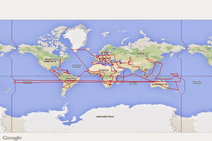
Using an algorithm to find a route from each country's capital to the remaining closest country's capital, I got the following route:

• Minimum Distance: 104,018 miles
• Minimum Route: United States of America, Canada, Bahamas, Cuba, Jamaica, Haiti, Dominican Republic, Saint Kitts and Nevis, Antigua and Barbuda, Dominica, Saint Lucia, Saint Vincent and the Grenadines, Grenada, Trinidad and Tobago, Barbados, Guyana, Suriname, Venezuela, Colombia, Ecuador, Panama, Costa Rica, Nicaragua, Honduras, El Salvador, Guatemala, Belize, Mexico, Peru, Bolivia, Paraguay, Uruguay, Argentina, Chile, Brazil, Cape Verde, Senegal, Gambia, Guinea-Bissau, Guinea, Sierra Leone, Liberia, Cote d'Ivoire, Ghana, Togo, Benin, Nigeria, Equatorial Guinea, Cameroon, Gabon, Sao Tome and Principe, Republic of the Congo, Democratic Republic of the Congo, Angola, Namibia, Botswana, South Africa, Swaziland, Mozambique, Lesotho, Zimbabwe, Zambia, Malawi, Tanzania, Kenya, Uganda, Rwanda, Burundi, South Sudan, Ethiopia, Djibouti, Yemen, Eritrea, Sudan, Egypt, Israel, Palestine, Jordan, Syria, Lebanon, Cyprus, Turkey, Romania, Bulgaria, Macedonia, Albania, Montenegro, Bosnia and Herzegovina, Serbia, Hungary, Slovakia, Austria, Czech Republic, Germany, Denmark, Norway, Sweden, Estonia, Finland, Latvia, Lithuania, Belarus, Ukraine, Moldova, Poland, Croatia, Slovenia, San Marino, Vatican City, Italy, Monaco, Switzerland, Liechtenstein, Luxembourg, Belgium, Netherlands, United Kingdom, France, Andorra, Spain, Portugal, Morocco, Algeria, Tunisia, Malta, Libya, Greece, Armenia, Georgia, Azerbaijan, Iran, Turkmenistan, Tajikistan, Uzbekistan, Kyrgyzstan, Kazakhstan, Afghanistan, Pakistan, India, Nepal, Bhutan, Bangladesh, Myanmar, Thailand, Laos, Viet Nam, Cambodia, Malaysia, Singapore, Indonesia, Brunei  Darussalam, Philippines, Taiwan, South Korea, North Korea, China, Mongolia, Japan, Palau, Timor-Leste, Papua New Guinea, Solomon Islands, Nauru, Kiribati, Marshall Islands, Micronesia, Tuvalu, Fiji, Tonga, Samoa, Vanuatu, New Zealand, Australia, Sri Lanka, Maldives, Seychelles, Somalia, Comoros, Madagascar, Mauritius, Oman, United Arab Emirates, Qatar, Bahrain, Saudi Arabia, Kuwait, Iraq, Russia, Ireland, Iceland, Greenland, Mauritania, Mali, Burkina Faso, Niger, Chad, Central African Republic

I had originally tried to manually visualize this route by plotting and drawing lines.  This was way too difficult and time consuming, so I figured there must be a better way using R.  Using RgoogleMaps, I came up with the following visualization:

This worked really well except when it came to the international dateline.  The plotting function interpreted the countries of Tonga and Samoa as being on the other side of the world from the other islands they are close to, because they have negative longitudes while the other islands have positive longitudes.  However, they are quite close geographically, which is why they were selected by the algorithm as being next in the route.  To fix this, I gave them a positive longitude by adding 360 to their actual longitude.  This corrected the problem visually.

For fun, I wrote a program to show the progression of the route from stop to stop.  Here is the result:

Happy travels!

Traveling State to State Using Simulation

Introduction

I know, I know... People have already blogged about the shortest/longest routes in traveling from state to state.  So nothing here is likely original.  But I thought I would do my own analysis with my own set of rules as a fun exercise in simulation.  Below is my method, my findings, and conclusions.

Method

I wrote an R program to simulate traveling from state to state.  I used the latitude/longitude for each state capital as the destination point in each state.  Always starting with the state of Washington (my home state), the program would then proceed to "move" from state to state until each state had been stopped in once and only once.  The program calculated the distance traveled "as the crow flies" between the states and then added it to the total.  The final output of the program listed the travel route (e.g., "Washington, Oregon, California,....") and the total mileage (e.g., 17650.37).

First Attempt: The Random Walk

My first program chose each successive state randomly.  I ran this simulation 100,000 times.  Here are the results:

• Minimum distance: 41,077 miles
• Minimum route: Washington, Oregon, Alaska, Hawaii, Arizona, California, Montana, New York, Connecticut, Idaho, Kansas, Mississippi, West Virginia, Wisconsin, Maryland, Wyoming, Utah, Ohio, Massachusetts, Rhode Island, North Carolina, New Jersey, Delaware, Florida, Louisiana, Oklahoma, Iowa, Minnesota, Indiana, Alabama, Tennessee, Nevada, Pennsylvania, Maine, Vermont, Kentucky, Colorado, Nebraska, New Mexico, New Hampshire, Virginia, South Dakota, North Dakota, South Carolina, Arkansas, Illinois, Georgia, Michigan, Missouri, Texas

• Maximum distance: 73,221 miles
• Maximum route: Washington, Indiana, South Dakota, Louisiana, West Virginia, Wisconsin, Montana, Florida, Connecticut, Alaska, Virginia, Oklahoma, Colorado, Pennsylvania, Wyoming, Delaware, Texas, Michigan, Massachusetts, Idaho, Vermont, South Carolina, Utah, New Hampshire, Nevada, Ohio, Arkansas, Kentucky, Mississippi, Nebraska, Alabama, New Mexico, Maryland, North Dakota, Illinois, Maine, New Jersey, California, Missouri, Minnesota, North Carolina, Hawaii, Rhode Island, Kansas, New York, Arizona, Iowa, Georgia, Oregon, Tennessee

• Average distance: 59,025 miles

Observations:

Given that we are choosing 50 states from 50 states (well, 49 from 49 since we start with Washington each time), there are 3 * 10^64 permutations of possible state to state routes available.  Even my simulation of 100,000 routes (supposing they are unique) covers only 1/(3 *10^60) possibilities.  That is practically 0%.  So the chances of stumbling across the "shortest" or "longest" routes randomly are pretty much non-existent. 

The "shortest" route randomly generated starts off well, staying largely on the west coast.  But then it jumps to New York and Connecticut, then back to Idaho.  It continues to jump to far off capitals when there are closer capitals available.  Similarly, the "longest" route does not always go to the farthest away capital.  Clearly, to find the "shortest" and "longest" routes we need give the computer guidance in selecting the next capital to visit.

Second Attempt: The Closest/Farthest State

I revised the program to always choose the closest state capital for the next stop.  As there is only one closest state capital to each state capital, there was only one possible route to take.  Similarly, I had the program select the farthest state capital for the next stop, resulting in one unique route.

• Minimum distance: 17,648 miles
• Minimum route: Washington, Oregon, Idaho, Montana, Utah, Wyoming, Colorado, New Mexico, Arizona, Nevada, California, South Dakota, North Dakota, Minnesota, Wisconsin, Illinois, Missouri, Kansas, Nebraska, Iowa, Indiana, Kentucky, Ohio, West Virginia, Virginia, Maryland, Delaware, New Jersey, Pennsylvania, New York, Connecticut, Rhode Island, Massachusetts, New Hampshire, Vermont, Maine, Michigan, Tennessee, Georgia, Alabama, Florida, South Carolina, North Carolina, Mississippi, Louisiana, Arkansas, Oklahoma, Texas, Alaska, Hawaii

To visualize this, here is a map:

• Maximum distance: 76,124 miles
• Maximum route: Washington, Hawaii, Maine, Alaska, Florida, Oregon, Massachusetts, California, Rhode Island, Nevada, New Hampshire, Arizona, Vermont, Idaho, Connecticut, Utah, New York, Montana, New Jersey, New Mexico, Delaware, Colorado, Maryland, Wyoming, Virginia, North Dakota, South Carolina, South Dakota, North Carolina, Texas, Pennsylvania, Oklahoma, West Virginia, Nebraska, Georgia, Minnesota, Louisiana, Michigan, Mississippi, Wisconsin, Alabama, Iowa, Ohio, Kansas, Kentucky, Arkansas, Indiana, Missouri, Tennessee, Illinois

Observations:
While the maximum route only increased by about 3,000 miles, the minimum route decreased by over 23,000 miles!  However, one can tell by looking at the map that this is clearly not the most efficient path to follow.  By selecting the closest capital, the program often got itself stuck in a corner and then had to jump a long distance to get to then next state capital.  Or it had to cross states it had already visited.  The jumps from California to South Dakota, Maine to Michigan, North Carolina to Mississippi, and Texas to Alaska make this very clear.

What this shows is that going to the closest state capital may not in fact lead to the shortest route overall.  In other words, it might make more sense to go to a capital a little farther away in order to shorten the overall route.  However, it is also obvious that at some point, going to a capital farther away will make the route longer.  For example, going to the capital farthest away most likely will not decrease the overall route distance.  So one should go to a capital that is close, but not the closest, in some cases to shorten the overall route...

Third Attempt: The Top n Closest States

To give the program more flexibility in selecting the next stop, I had it find the top n closest states, and then it chose randomly from that set for it's next stop.  For example, if it was finding the top 2 closest states for Washington, it would find Oregon and Idaho and randomly choose one or the other.  Some routes started with "Washington, Oregon,...." while others started with "Washington, Idaho,...".  In this way, the program could go to a state that was close, but not always the closest, in hopes of shortening the overall route. Using the top 2 closest states produced the best results.   I ran this simulation 100,000 times.

For n=2:

• Minimum distance: 16,245 miles
• Average distance: 22,360 miles
• Minimum route: Washington, Idaho, Utah, Wyoming, Colorado, South Dakota, North Dakota, Minnesota, Iowa, Nebraska, Kansas, Missouri, Illinois, Wisconsin, Michigan, Indiana, Kentucky, Ohio, West Virginia, North Carolina, Virginia, Maryland, Delaware, Pennsylvania, New Jersey, Connecticut, New York, New Hampshire, Massachusetts, Rhode Island, Vermont, Maine, Tennessee, Alabama, Florida, Georgia, South Carolina, Louisiana, Mississippi, Arkansas, Oklahoma, Texas, New Mexico, Arizona, Nevada, California, Montana, Oregon, Alaska, Hawaii

To visualize...

Observations:
While on average, these routes were longer than always going to the closest state, on occasion they were shorter.  The shortest route by this method was 1,400 miles shorter than the previous method.  The shortest routes all circled around the United States, either along the top or the bottom going east, and then came back west on the opposite side as going east.  Finally, they all went to Alaska and then ended with Hawaii.  This makes sense as it means that very little ground is covered twice, and the states farthest away are left for last and are reached by the closest remaining states.

Still, one can see from the map that there are some inefficiencies, lines crossed, states covered twice, etc.  So it is not perfect...

Fourth Attempt: Bubble Sort Style Algorithm

I combined the previous attempts into a bubble sort style algorithm.  I had the computer generate a route randomly and then calculate the total mileage. I then had the program swap states and recalculate the mileage.  If the mileage decreased, the new route was kept, and the process was repeated.  The program did this until every possible state swap had been attempted and no more swaps occurred.  That is, no more swapping could reduce the total mileage.  Then the final route was output.  I ran this simulation 1,500 times each for the shortest and longest routes.

• Minimum distance: 15,173 miles
• Average distance: 19,760 miles
• Minimum route: Washington, Oregon, Idaho, Nevada, California, Arizona, Texas, Oklahoma, Kansas, Nebraska, Iowa, Missouri, Arkansas, Mississippi, Louisiana, Alabama, Florida, Georgia, Tennessee, Kentucky, West Virginia, South Carolina, North Carolina, Virginia, Maryland, Delaware, Pennsylvania, New Jersey, Connecticut, Rhode Island, Massachusetts, New Hampshire, Maine, Vermont, New York, Michigan, Ohio, Indiana, Illinois, Wisconsin, Minnesota, North Dakota, South Dakota, Wyoming, Colorado, New Mexico, Utah, Montana, Alaska, Hawaii

• Maximum distance: 81,927 miles
• Average distance: 81,240 miles
• Maximum route: Washington, North Carolina, Idaho, Virginia, Nebraska, Rhode Island, Arizona, Massachusetts, Illinois, Arkansas, Vermont, Oklahoma, New Hampshire, Missouri, New York, New Mexico, Connecticut, Colorado, Pennsylvania, Hawaii, Delaware, Nevada, Maryland, Wyoming, West Virginia, Oregon, Kentucky, Montana, South Carolina, South Dakota, Tennessee, Alaska, Georgia, Iowa, Florida, North Dakota, Alabama, Minnesota, Mississippi, Wisconsin, Louisiana, Michigan, Texas, Maine, Kansas, New Jersey, California, Ohio, Utah, Indiana

Observations:
This method was a great improvement over the previous methods.  The total mileage decreased on average and the shortest route was 1,100 miles shorter than the previous shortest route.  This route also had no crisscrossing of paths, the first time I had seen this occur (and which would be expected in the shortest route possible).  The longest route of 81,927miles  was 5,803 miles longer than the previous record of 76,124 miles.  All in all, this method was much better than prior attempts.

 Fifth Attempt: Insertion Sort Style Algorithm

The previous attempt, despite being very successful, was incredibly slow.  It took over 12 hours to get 1,500 results.  If I wanted to do a larger simulation, I would need to have a faster algorithm.  Also, being so close to breaking 15,000 miles, I wanted to see if there was a route that was in the 14,000s.  Similarly, being so close to 82,000 miles, I wanted to see if there was a longest route that was in the 82,000s.

I knew bubble sort wasn't the fastest algorithm, so I looked at other sorting algorithms to determine which would be best for my problem.  It seemed that insertion sort was going to be the best and most appropriate for my needs, so I rewrote the program to use insertion sort.  The program created a route randomly.  It then took a given state and inserted it into each other possible position in the route.  If the mileage decreased, the insertion was kept, and the program moved on to the next state.  When it got to the end of the route, it repeated the process starting at the beginning of the updated route.  This was done until no more insertion changes were made.  Then the final route and mileage was output.  The time a complete process took did not decrease dramatically, so I did 500 simulations each for finding the longest and shortest routes.

• Minimum distance:  14,589 miles
• Average distance: 16, 156 miles
• Minimum route: Washington, Oregon, California, Nevada, Idaho, Utah, Arizona, New Mexico, Colorado, Wyoming, Oklahoma, Texas, Louisiana, Mississippi, Arkansas, Missouri, Illinois, Indiana, Ohio, West Virginia, Kentucky, Tennessee, Georgia, Alabama, Florida, South Carolina, North Carolina, Virginia, Maryland, Delaware, New Jersey, Connecticut, Rhode Island, Massachusetts, New Hampshire, Maine, Vermont, New York, Pennsylvania, Michigan, Wisconsin, Minnesota, Iowa, Kansas, Nebraska, South Dakota, North Dakota, Montana, Alaska, Hawaii

• Maximum distance: 80,576 miles
• Average distance: 79,634 miles
• Maximum route: Washington, Florida, South Dakota, Tennessee, Alaska, Georgia, Minnesota, Alabama, Wisconsin, Oklahoma, Indiana, Texas, Michigan, Louisiana, North Dakota, Mississippi, Maine, Nebraska, Connecticut, Missouri, Rhode Island, Hawaii, Ohio, Kansas, South Carolina, Idaho, Delaware, Nevada, New York, Wyoming, New Jersey, Colorado, Maryland, California, North Carolina, Montana, Massachusetts, New Mexico, Virginia, Utah, West Virginia, Iowa, Vermont, Oregon, Kentucky, Arizona, New Hampshire, Arkansas, Pennsylvania, Illinois

Insertion sort didn't work so well for finding the longest route, so I tried the bubble sort method again, simply to try and break 82,000 miles.  After 1,000 simulations, it still hadn't broken 82,000 and had only improved by 1 mile.

• Maximum distance: 81,928 miles
• Maximum route: Washington, Kentucky, Utah, Pennsylvania, Kansas, Massachusetts, Arizona, Rhode Island, Nebraska, Tennessee, Iowa, Ohio, California, Maryland, Nevada, Virginia, Idaho, Indiana, Texas, Vermont, Arkansas, Michigan, Louisiana, Wisconsin, Mississippi, Minnesota, Alabama, North Dakota, Florida, Alaska, Georgia, South Dakota, South Carolina, Montana, North Carolina, Oregon, West Virginia, Wyoming, New York, Oklahoma, Maine, Missouri, New Jersey, Hawaii, Delaware, Colorado, Connecticut, New Mexico, New Hampshire, Illinois

Observations:
While my simulation easily broke into the 14,000s, it could not break into the 82,000s.  Perhaps with more time, more computing power, and a further refined algorithm this would eventually happen.  But a large gain in either direction was very unlikely at this point, so I decided to be content with my findings.

 Conclusion

The shortest route from state capital to state capital seems to be about 14,500 miles, while the longest route seems to be about 82,000 miles.  I'm sure that a shorter route exists than what I found, but this is not likely to be much shorter given that very few miles were gained in these final attempts.  As for the longer route, there probably is a slightly longer route, but I am skeptical that one can break 82,000 miles.  However, I'd be happy to be proven wrong...

Overall, this exercise shows that simulation is a very powerful tool in solving problems, particularly when implemented well (i.e., goal directed and iterative).

Happy travels!